Predicting Supply Chain Disruptions

In a previous post, I have introduced the concept of Temporal Multi-Party Analysis (TEMPA) graphs as a model for understanding the behaviour of complex connected networks.

In this post, I will share a detailed example of how TEMPA model can be used to analyze supply chain disruptions and risk of shortage for generic drugs.

Generic Drug Supply Chains: A Complex & Evolving Landscape

In the past decade, the public in many countries have become increasingly aware of the persistent problem of severe drug shortages and this issue has been further amplified during periods of emergency.

Due to the interconnected economic dynamics of the pharmaceutical market, complex and fragmented global supply chains and stringent regulatory good manufacturing practice (GMP) requirements, the behaviour of demand and supply systems for prescription drugs, especially generic drugs, follows some non-intuitive patterns when supply disruptions happen.

While supply disruptions lead to drug shortages and an increase in demand, even a subsequent increase in prices, in the case of generic drugs, this trigger does not seem to follow the normal economic theory of acting as an incentive for existing and new suppliers to increase production to meet the demand. A key factor for this disincentive is the pricing dynamic created by group purchasing of generic drugs.

While single-payer healthcare systems followed in Canada, United Kingdom, Australia and most European Union countries have traditionally relied on consolidated procurement and government shared service organizations (SSO), the US healthcare market has also been shifting rapidly towards a group procurement model with Pharmacy & Therapeutics (P&T) Committees and Group Purchasing Organizations (GPO) driving large scale and bulk sourcing decisions.

These volume and pricing dynamics consequently shape the supply chains, vendors and markets for medical products, specifically generic drug products.

Due to the downward cost pressure created by bulk procurement and loss of patent protection, there has been a growing concentration of raw material or generic Active Pharmaceutical Ingredient (API) supply in sole-source suppliers and low-cost manufacturing locations such as China and India.

The concentration of supply in limited suppliers and the drive to reduce cost creates knock-on risks in the system. In the absence of any premium or market compensation for quality management, the fragility of the supply chain to quality control or manufacturing breakdowns is greatly increased. If the market supplier is the ‘sole-source’ for specific APIs (active pharmaceutical ingredients) then the regulatory requirements for switching suppliers or rapidly building capacity is also greatly hindered.

With supply chains coupled tightly and distributed globally across multiple geographies, the ability to switch suppliers, build new facilities or modify existing facilities also requires multiple regulatory approvals which further constrains the ability of manufacturers to quickly adjust production volumes after a supply disruption has occurred.

Application of TEMPA to predict sustained supply disruptions

A Temporal Multi-Party Analysis (TEMPA) model can be utilized to understand, visualize and model the demand and supply dynamics of different generic drugs over time, revealing the triggers that lead to persistent supply disruptions and result in shortages of specific generic drugs.

The example below will model a simplified and hypothetical demand and supply system for Hydroxychloroquine which is used in the treatment of malaria, lupus and rheumatoid arthritis.

We assume here that the active pharmaceutical ingredient (API) is being used to produce a rheumatoid arthritis branded product P3 by a major pharmaceutical BP at their manufacturing plant M3.

The API is also being used by two generic manufacturers GM1 and GM2, who produce generic drug products P1 for Malaria and P2 for Lupus at their plants M1 and M2 respectively.

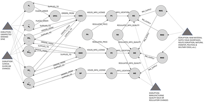
The following entities are included in the graph to show additional system dynamics.

H1…H5 — healthcare entities that prescribe or approve the inclusion of products P1 and P2 in clinical practice. This includes hospitals, long term care homes, etc.

GPO1 — group procurement entity that purchases from GM1 on behalf of H1…H5 and their Shared Service Organizations (SSOs).

PH1…PH10 and PC1…PC20 — these are several other healthcare entities such as pharmacies and primary care clinics that purchase directly from both GM1 and GM2.

M1 and M2 — manufacturing sites in India for GM1 and GM2 respectively.

RM1, RM2 and RM3 — raw material suppliers in China that supply to M1, M2 and M3.

RA — healthcare regulatory authority in the market where P1 and P2 are distributed.

PA — Government Insurance or Payer Agency that drives financing arrangements and price controls for manufacturing and distribution of generic products P1 and P2.

A high-level topography in Figure 1 below, shows an illustrative graph of how the different entities relate to each other and the nodes that will be directly impacted in case of disruptions.

As different disruptions influence the demand-supply dynamic of the system, they in turn impact the likelihood of creating sustained supply disruptions. Not all supply disruptions lead to shortages, since actions can be taken in between that prevent the onset of a shortage, but nearly all shortages are preceded by supply disruptions.

If a supply disruption persists, it becomes a drug shortage, an extended period in which existing and new suppliers are unable to increase production enough to meet demand.

Assuming that the main focus of Temporal Multi-Party Analysis (TEMPA) is to model the dependencies between the demand and supply nodes of the product P1, specifically how disruptions at any of the nodes propagate across the system over time. This will help predict the likelihood of sustained supply disruptions which is a leading indicator for shortages. Using the TEMPA model specification introduced earlier, we will model the system over a rolling three-month period, as below.

For the model, let’s assume Î = {1,2,3, … ,90} is a set of discrete daily intervals over 90 days. The time interval t belongs to Î.

P (t)(i) is the weight or influence of node i at time t. Assuming the influence is constant over Î, we will denote the property of node i as P(i) where,

For supply nodes, P(i)= (node’s contribution to 90-day supply) / total 90-day supply

For demand nodes, P(i)= (node’s contribution to 90-day demand) / total 90-day demand

Š (t)(i) is the direct disruption of node i at time t. Internal and external events create disruption which first impacts certain nodes directly and then ripples over time through the system to other nodes.

Using natural language processing (NLP) and trained machine learning (ML) algorithms, we can classify events from an environmental scan at time t, creating a list of impacts on the different demand and supply nodes in the graph. This type of event monitoring auto-classifies events and assigns category, node, impact and duration scores, based on prior training data.

The environmental scan includes monitoring of news sources (political factors, natural disasters, epidemics, seasonal demand, health trends, etc.), regulatory body databases (FDA Inspections Database, FDA 483 citations, etc.), pharma industry reports, hospital and public health databases.

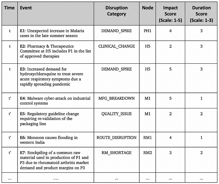
In the scoring framework above, Impact Scores are assigned to different events by classifying them across a range of impact (1 lowest — 5 highest), based on similarity to prior events and their scope and disruption on the supply of product P1.

Duration Scores are assigned based on how long the disruptive effect of the event is expected to last (30 days : 1 | 60 days : 2 | 90 days : 3).

The direct disruption state of a node i that is impacted by k events at time t is calculated as,

The weighted disruption that is transmitted between nodes is based on the property of the node (defined as its weight/influence) and the state of the node (total disruption). The weighted transmission from node i to node j at time t is calculated as,

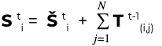
The state (disruption score) of a node i is therefore determined by the effect of direct disruption at time t and the effect of transmitted disruptions from all connections in an N node graph at t-1.

The state or the supply disruption score for all the entities in the graph evolves in time as impacts from different events accumulate or dissipate disruption scores on the different nodes. The entities that accumulate the highest scores are the most vulnerable points in the system.

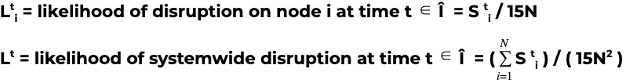
Likelihood is calculated as a ratio of the disruption score at time t divided by the maximum possible disruption score if the graph was a fully connected graph. This gives us the following probabilities for a graph with N nodes.

The system trends for a supply disruption can be through a time phased graph and node heat map for the values of L (t)(i) and observing L (t) for the overall system provides signals for early intervention and may be used to reduce the risk of sustained supply disruption and subsequent shortages.

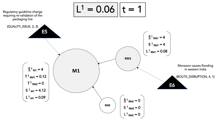
In order to illustrate how this model would work, an example is provided in Figures 2 and 3 below.

For the sake of simplicity, the example only includes the three supply nodes — manufacturing plant M1 and the raw material suppliers RM1 and RM2 from the demand-supply topography of drug product P1. This directed graph has three nodes, so N = 3.

The nodes sizes are proportional to their property P(i) or the influence weight of each node on supply. Events E5 and E6 occur at time t = 1 leading to different direct and transmitted disruption scores on each node and different likelihoods (0 ⩽ L(t)(i) ⩽ 1) of disruption. The grayscale shade of the node is representative of the disruption likelihood on each node.

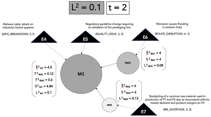
At time t = 2, two additional events E4 and E7 impact the nodes and this leads to additional accumulation of disruption scores across the nodes and we can see that the likelihood of disruption on M1 and the overall disruption likelihood L(t) is increasing rapidly.

Conclusion

Elaborating this Temporal Multi-Party Analysis (TEMPA) model over additional time periods and events, taking into account the full topography that includes both demand nodes and supply nodes, will provide a visual heat map to see impending supply disruption risks and help in the identification of risky nodes that may require specific interventions to prevent sustained disruption and subsequent shortage of the generic drug product P1.

While the example provided here is for supply disruption of generic drugs, it can be easily extended to other sectors with the TEMPA model providing a robust framework for analyzing the end-to-end system and predicting disruptions, bottlenecks and risks in any complex supply chain.

References

1. S. Wagner et al. (2009) Assessing the vulnerability of supply chains using graph theory

2. P. Gai et al. (2011) Complexity, concentration and contagion

3. J. Duffin (2020) Canada drug shortage site www.canadadrugshortage.com

4. U.S. FDA (2019) Drug Shortages: Root Causes and Potential Solutions

5. M. Y. Naghmouchi et al. (2016) A New Risk Assessment Framework Using Graph Theory